Single-phase power systems

Single-phase

                            

Depicted above is a very simple AC circuit. If the load resistor's power dissipation were substantial, we might call this a "power circuit" or "power system" instead of regarding it as just a regular circuit. The distinction between a "power circuit" and a "regular circuit" may seem arbitrary, but the practical concerns are definitely not.
One such concern is the size and cost of wiring necessary to deliver power from the AC source to the load. Normally, we do not give much thought to this type of concern if we're merely analyzing a circuit for the sake of learning about the laws of electricity. However, in the real world it can be a major concern. If we give the source in the above circuit a voltage value and also give power dissipation values to the two load resistors, we can determine the wiring needs for this particular circuit:

83.33 amps for each load resistor adds up to 166.66 amps total circuit current. This is no small amount of current, and would necessitate copper wire conductors of at least 1/0 gage. Such wire is well over 1/4 inch in diameter, weighing over 300 pounds per thousand feet. Bear in mind that copper is not cheap either! It would be in our best interest to find ways to minimize such costs if we were designing a power system with long conductor lengths.
One way to do this would be to increase the voltage of the power source and use loads built to dissipate 10 kW each at this higher voltage. The loads, of course, would have to have greater resistance values to dissipate the same power as before (10 kW each) at a greater voltage than before. The advantage would be less current required, permitting the use of smaller, lighter, and cheaper wire:

Now our total circuit current is 83.33 amps, half of what it was before. We can now use number 4 gage wire, which weighs less than half of what 1/0 gage wire does per unit length. This is a considerable reduction in system cost with no degradation in performance. This is why power distribution system designers elect to transmit electric power using very high voltages (many thousands of volts): to capitalize on the savings realized by the use of smaller, lighter, cheaper wire.
However, this solution is not without disadvantages. Another practical concern with power circuits is the danger of electric shock from high voltages. Again, this is not usually the sort of thing we concentrate on while learning about the laws of electricity, but it is a very valid concern in the real world, especially when large amounts of power are being dealt with. The gain in efficiency realized by stepping up the circuit voltage presents us with increased danger of electric shock. Power distribution companies tackle this problem by stringing their power lines along high poles or towers, and insulating the lines from the supporting structures with large, porcelain insulators.
At the point of use (the electric power customer), there is still the issue of what voltage to use for powering loads. High voltage gives greater system efficiency by means of reduced conductor current, but it might not always be practical to keep power wiring out of reach at the point of use the way it can be elevated out of reach in distribution systems. This tradeoff between efficiency and danger is one that European power system designers have decided to risk, all their households and appliances operating at a nominal voltage of 240 volts instead of 120 volts as it is in North America. That is why tourists from America visiting Europe must carry small step-down transformers for their portable appliances, to step the 240 VAC (volts AC) power down to a more suitable 120 VAC.
Is there any way to realize the advantages of both increased efficiency and reduced safety hazard at the same time? One solution would be to install step-down transformers at the end-point of power use, just as the American tourist must do while in Europe. However, this would be expensive and inconvenient for anything but very small loads (where the transformers can be built cheaply) or very large loads (where the expense of thick copper wires would exceed the expense of a transformer).
An alternative solution would be to use a higher voltage supply to provide power to two lower voltage loads in series. This approach combines the efficiency of a high-voltage system with the safety of a low-voltage system:

Voltage "polarity," AC Polarity, AC Polarity, AC
Notice the polarity markings (+ and -) for each voltage shown, as well as the unidirectional arrows for current. For the most part, I've avoided labeling "polarities" in the AC circuits we've been analyzing, even though the notation is valid to provide a frame of reference for phase. In later sections of this chapter, phase relationships will become very important, so I'm introducing this notation early on in the chapter for your familiarity.
The current through each load is the same as it was in the simple 120 volt circuit, but the currents are not additive because the loads are in series rather than parallel. The voltage across each load is only 120 volts, not 240, so the safety factor is better. Mind you, we still have a full 240 volts across the power system wires, but each load is operating at a reduced voltage. If anyone is going to get shocked, the odds are that it will be from coming into contact with the conductors of a particular load rather than from contact across the main wires of a power system.
There's only one disadvantage to this design: the consequences of one load failing open, or being turned off (assuming each load has a series on/off switch to interrupt current) are not good. Being a series circuit, if either load were to open, current would stop in the other load as well. For this reason, we need to modify the design a bit:
Hot conductor Neutral conductor

Split-phase
Instead of a single 240 volt power supply, we use two 120 volt supplies (in phase with each other!) in series to produce 240 volts, then run a third wire to the connection point between the loads to handle the eventuality of one load opening. This is called a split-phase power system. Three smaller wires are still cheaper than the two wires needed with the simple parallel design, so we're still ahead on efficiency. The astute observer will note that the neutral wire only has to carry the difference of current between the two loads back to the source. In the above case, with perfectly "balanced" loads consuming equal amounts of power, the neutral wire carries zero current.
Notice how the neutral wire is connected to earth ground at the power supply end. This is a common feature in power systems containing "neutral" wires, since grounding the neutral wire ensures the least possible voltage at any given time between any "hot" wire and earth ground.
An essential component to a split-phase power system is the dual AC voltage source. Fortunately, designing and building one is not difficult. Since most AC systems receive their power from a step-down transformer anyway (stepping voltage down from high distribution levels to a user-level voltage like 120 or 240), that transformer can be built with a center-tapped secondary winding:

If the AC power comes directly from a generator (alternator), the coils can be similarly center-tapped for the same effect. The extra expense to include a center-tap connection in a transformer or alternator winding is minimal.
Boosting, AC voltage sources Bucking, AC voltage sources
Here is where the (+) and (-) polarity markings really become important. This notation is often used to reference the phasings of multiple AC voltage sources, so it is clear whether they are aiding ("boosting") each other or opposing ("bucking") each other. If not for these polarity markings, phase relations between multiple AC sources might be very confusing. Note that the split-phase sources in the schematic (each one 120 volts0^o), with polarity marks (+) to (-) just like series-aiding batteries can alternatively be represented as such:

To mathematically calculate voltage between "hot" wires, we must subtract voltages, because their polarity marks show them to be opposed to each other:

If we mark the two sources' common connection point (the neutral wire) with the same polarity mark (-), we must express their relative phase shifts as being 180^o apart. Otherwise, we'd be denoting two voltage sources in direct opposition with each other, which would give 0 volts between the two "hot" conductors. Why am I taking the time to elaborate on polarity marks and phase angles? It will make more sense in the next section!
Single-phase
Power systems in American households and light industry are most often of the split-phase variety, providing so-called 120/240 VAC power. The term "split-phase" merely refers to the split-voltage supply in such a system. In a more general sense, this kind of AC power supply is called single phase because both voltage waveforms are in phase, or in step, with each other.
The term "single phase" is a counterpoint to another kind of power system called "polyphase" which we are about to investigate in detail. Apologies for the long introduction leading up to the title-topic of this chapter. The advantages of polyphase power systems are more obvious if one first has a good understanding of single phase systems.

Review

Single phase power systems are defined by having an AC source with only one voltage waveform. A split-phase power system is one with multiple (in-phase) AC voltage sources connected in series, delivering power to loads at more than one voltage, with more than two wires. They are used primarily to achieve balance between system efficiency (low conductor currents) and safety (low load voltages). Split-phase AC sources can be easily created by center-tapping the coil windings of transformers or alternators.

Harmonic phase sequences

  Triplen harmonics 

In the last section, we saw how the 3rd harmonic and all of its integer multiples (collectively called triplenharmonics) generated by 120^o phase-shifted fundamental waveforms are actually in phase with each other. In a 60 Hz three-phase power system, where phases A, B, and C are 120^o apart, the third-harmonic multiples of those frequencies (180 Hz) fall perfectly into phase with each other. This can be thought of in graphical terms, and/or in mathematical terms:

If we extend the mathematical table to include higher odd-numbered harmonics, we will notice an interesting pattern develop with regard to the rotation or sequence of the harmonic frequencies:

Positive sequence Negative sequence Zero sequence Harmonic sequence Sequence, harmonic

Harmonics such as the 7th, which "rotate" with the same sequence as the fundamental, are called positive sequence. Harmonics such as the 5th, which "rotate" in the opposite sequence as the fundamental, are called negative sequence. Triplen harmonics (3rd and 9th shown in this table) which don't "rotate" at all because they're in phase with each other, are called zero sequence.

This pattern of positive-zero-negative-positive continues indefinitely for all odd-numbered harmonics, lending itself to expression in a table like this:

Sequence especially matters when we're dealing with AC motors, since the mechanical rotation of the rotor depends on the torque produced by the sequential "rotation" of the applied 3-phase power. Positive-sequence frequencies work to push the rotor in the proper direction, whereas negative-sequence frequencies actually work against the direction of the rotor's rotation. Zero-sequence frequencies neither contribute to nor detract from the rotor's torque. An excess of negative-sequence harmonics (5th, 11th, 17th, and/or 23rd) in the power supplied to a three-phase AC motor will result in a degradation of performance and possible overheating. Since the higher-order harmonics tend to be attenuated more by system inductances and magnetic core losses, and generally originate with less amplitude anyway, the primary harmonic of concern is the 5th, which is 300 Hz in 60 Hz power systems and 250 Hz in 50 Hz power systems.

Standing waves and resonance/Transmission line-part F

Standing waves and resonance

Standing waves

Whenever there is a mismatch of impedance between transmission line and load, reflections will occur. If the incident signal is a continuous AC waveform, these reflections will mix with more of the oncoming incident waveform to produce stationary waveforms called standing waves.

The following illustration shows how a triangle-shaped incident waveform turns into a mirror-image reflection upon reaching the line's unterminated end. The transmission line in this illustrative sequence is shown as a single, thick line rather than a pair of wires, for simplicity's sake. The incident wave is shown traveling from left to right, while the reflected wave travels from right to left:

Wave guides/Transmission line-part-H

Wave-guides

A waveguide is a special form of transmission line consisting of a hollow, metal tube. The tube wall provides distributed inductance, while the empty space between the tube walls provide distributed capacitance:

Long and Short Transmission Lines-Transmission line PART-E

Long and Short Transmission Lines

In DC and low-frequency AC circuits, the characteristic impedance of parallel wires is usually ignored. This includes the use of coaxial cables in instrument circuits, often employed to protect weak voltage signals from being corrupted by induced "noise" caused by stray electric and magnetic fields. This is due to the relatively short time spans in which reflections take place in the line, as compared to the period of the waveform or pulses of the significant signals in the circuit. As we saw in the last section, if a transmission line is connected to a DC voltage source, it will behave as a resistor equal in value to the line's characteristic impedance only for as long as it takes the incident pulse to reach the end of the line and return as a reflected pulse, back to the source. After that time (a brief 16.292 μs for the mile-long coaxial cable of the last example), the source "sees" only the terminating impedance, whatever that may be.

If the circuit in question handles low-frequency AC power, such short time delays introduced by a transmission line between when the AC source outputs a voltage peak and when the source "sees" that peak loaded by the terminating impedance (round-trip time for the incident wave to reach the line's end and reflect back to the source) are of little consequence. Even though we know that signal magnitudes along the line's length are not equal at any given time due to signal propagation at (nearly) the speed of light, the actual phase difference between start-of-line and end-of-line signals is negligible, because line-length propagation occur within a very small fraction of the AC waveform's period. For all practical purposes, we can say that voltage along all respective points on a low-frequency, two-conductor line are equal and in-phase with each other at any given point in time.

In these cases, we can say that the transmission lines in question are electrically short, because their propagation effects are much quicker than the periods of the conducted signals. By contrast, an electrically long line is one where the propagation time is a large fraction or even a multiple of the signal period. A "long" line is generally considered to be one where the source's signal waveform completes at least a quarter-cycle (90o of "rotation") before the incident signal reaches line's end. Up until this chapter in the Lessons In Electric Circuits book series, all connecting lines were assumed to be electrically short.

To put this into perspective, we need to express the distance traveled by a voltage or current signal along a transmission line in relation to its source frequency. An AC waveform with a frequency of 60 Hz completes one cycle in 16.66 ms. At light speed (186,000 m/s), this equates to a distance of 3100 miles that a voltage or current signal will propagate in that time. If the velocity factor of the transmission line is less than 1, the propagation velocity will be less than 186,000 miles per second, and the distance less by the same factor. But even if we used the coaxial cable's velocity factor from the last example (0.66), the distance is still a very long 2046 miles! Whatever distance we calculate for a given frequency is called the wavelength of the signal.

The lower-case Greek letter "lambda" (λ) represents wavelength, in whatever unit of length used in the velocity figure (if miles per second, then wavelength in miles; if meters per second, then wavelength in meters). Velocity of propagation is usually the speed of light when calculating signal wavelength in open air or in a vacuum, but will be less if the transmission line has a velocity factor less than 1.

If a "long" line is considered to be one at least 1/4 wavelength in length, you can see why all connecting lines in the circuits discussed thusfar have been assumed "short." For a 60 Hz AC power system, power lines would have to exceed 775 miles in length before the effects of propagation time became significant. Cables connecting an audio amplifier to speakers would have to be over 4.65 miles in length before line reflections would significantly impact a 10 kHz audio signal!

When dealing with radio-frequency systems, though, transmission line length is far from trivial. Consider a 100 MHz radio signal: its wavelength is a mere 9.8202 feet, even at the full propagation velocity of light (186,000 m/s). A transmission line carrying this signal would not have to be more than about 2-1/2 feet in length to be considered "long!" With a cable velocity factor of 0.66, this critical length shrinks to 1.62 feet.

When an electrical source is connected to a load via a "short" transmission line, the load's impedance dominates the circuit. This is to say, when the line is short, its own characteristic impedance is of little consequence to the circuit's behavior. We see this when testing a coaxial cable with an ohmmeter: the cable reads "open" from center conductor to outer conductor if the cable end is left unterminated. Though the line acts as a resistor for a very brief period of time after the meter is connected (about 50 Ω for an RG-58/U cable), it immediately thereafter behaves as a simple "open circuit:" the impedance of the line's open end. Since the combined response time of an ohmmeter and the human being using it greatly exceeds the round-trip propagation time up and down the cable, it is "electrically short" for this application, and we only register the terminating (load) impedance. It is the extreme speed of the propagated signal that makes us unable to detect the cable's 50 Ω transient impedance with an ohmmeter.

If we use a coaxial cable to conduct a DC voltage or current to a load, and no component in the circuit is capable of measuring or responding quickly enough to "notice" a reflected wave, the cable is considered "electrically short" and its impedance is irrelevant to circuit function. Note how the electrical "shortness" of a cable is relative to the application: in a DC circuit where voltage and current values change slowly, nearly any physical length of cable would be considered "short" from the standpoint of characteristic impedance and reflected waves. Taking the same length of cable, though, and using it to conduct a high-frequency AC signal could result in a vastly different assessment of that cable's "shortness!"

When a source is connected to a load via a "long" transmission line, the line's own characteristic impedance dominates over load impedance in determining circuit behavior. In other words, an electrically "long" line acts as the principal component in the circuit, its own characteristics overshadowing the load's. With a source connected to one end of the cable and a load to the other, current drawn from the source is a function primarily of the line and not the load. This is increasingly true the longer the transmission line is. Consider our hypothetical 50 Ω cable of infinite length, surely the ultimate example of a "long" transmission line: no matter what kind of load we connect to one end of this line, the source (connected to the other end) will only see 50 Ω of impedance, because the line's infinite length prevents the signal from ever reaching the end where the load is connected. In this scenario, line impedance exclusively defines circuit behavior, rendering the load completely irrelevant.

The most effective way to minimize the impact of transmission line length on circuit behavior is to match the line's characteristic impedance to the load impedance. If the load impedance is equal to the line impedance, then anysignal source connected to the other end of the line will "see" the exact same impedance, and will have the exact same amount of current drawn from it, regardless of line length. In this condition of perfect impedance matching, line length only affects the amount of time delay from signal departure at the source to signal arrival at the load. However, perfect matching of line and load impedance is not always practical or possible.

The next section discusses the effects of "long" transmission lines, especially when line length happens to match specific fractions or multiples of signal wavelength.
Review
Coaxial cabling is sometimes used in DC and low-frequency AC circuits as well as in high-frequency circuits, for the excellent immunity to induced "noise" that it provides for signals. 

When the period of a transmitted voltage or current signal greatly exceeds the propagation time for a transmission line, the line is considered electrically short. Conversely, when the propagation time is a large fraction or multiple of the signal's period, the line is considered electrically long. 

A signal's wavelength is the physical distance it will propagate in the time span of one period. 

Wavelength is calculated by the formula λ=v/f, where "λ" is the wavelength, "v" is the propagation velocity, and "f" is the signal frequency. 

A rule-of-thumb for transmission line "shortness" is that the line must be at least 1/4 wavelength before it is considered "long." 

In a circuit with a "short" line, the terminating (load) impedance dominates circuit behavior. The source effectively sees nothing but the load's impedance, barring any resistive losses in the transmission line. 

In a circuit with a "long" line, the line's own characteristic impedance dominates circuit behavior. The ultimate example of this is a transmission line of infinite length: since the signal will never reach the load impedance, the source only "sees" the cable's characteristic impedance. 

When a transmission line is terminated by a load precisely matching its impedance, there are no reflected waves and thus no problems with line length.

Read More About

Circuit Schematic Symbols

Transmission line- 50-Ohm Cable- Part-A

Transmission line-Circuits and the speed of light-Part-B

Transmission line-Characteristic impedance-part-c

Finite-length transmission lines-Part-D

Finite-length transmission lines-Part-D

Finite-length transmission lines

A transmission line of infinite length is an interesting abstraction, but physically impossible. All transmission lines have some finite length, and as such do not behave precisely the same as an infinite line. If that piece of 50 Ω "RG-58/U" cable I measured with an ohmmeter years ago had been infinitely long, I actually would have been able to measure 50 Ω worth of resistance between the inner and outer conductors. But it was not infinite in length, and so it measured as "open" (infinite resistance).
Nonetheless, the characteristic impedance rating of a transmission line is important even when dealing with limited lengths. An older term for characteristic impedance, which I like for its descriptive value, is surge impedance. If a transient voltage (a "surge") is applied to the end of a transmission line, the line will draw a current proportional to the surge voltage magnitude divided by the line's surge impedance (I=E/Z). This simple, Ohm's Law relationship between current and voltage will hold true for a limited period of time, but not indefinitely.
If the end of a transmission line is open-circuited -- that is, left unconnected  the current "wave" propagating down the line's length will have to stop at the end, since electrons cannot flow where there is no continuing path. This abrupt cessation of current at the line's end causes a "pile-up" to occur along the length of the transmission line, as the electrons successively find no place to go. Imagine a train traveling down the track with slack between the rail car couplings: if the lead car suddenly crashes into an immovable barricade, it will come to a stop, causing the one behind it to come to a stop as soon as the first coupling slack is taken up, which causes the next rail car to stop as soon as the next coupling's slack is taken up, and so on until the last rail car stops. The train does not come to a halt together, but rather in sequence from first car to last:

A signal propagating from the source-end of a transmission line to the load-end is called an incident wave. The propagation of a signal from load-end to source-end (such as what happened in this example with current encountering the end of an open-circuited transmission line) is called a reflected wave.
When this electron "pile-up" propagates back to the battery, current at the battery ceases, and the line acts as a simple open circuit. All this happens very quickly for transmission lines of reasonable length, and so an ohmmeter measurement of the line never reveals the brief time period where the line actually behaves as a resistor. For a mile-long cable with a velocity factor of 0.66 (signal propagation velocity is 66% of light speed, or 122,760 miles per second), it takes only 1/122,760 of a second (8.146 microseconds) for a signal to travel from one end to the other. For the current signal to reach the line's end and "reflect" back to the source, the round-trip time is twice this figure, or 16.292 μs.
High-speed measurement instruments are able to detect this transit time from source to line-end and back to source again, and may be used for the purpose of determining a cable's length. This technique may also be used for determining the presence and location of a break in one or both of the cable's conductors, since a current will "reflect" off the wire break just as it will off the end of an open-circuited cable. Instruments designed for such purposes are called time-domain reflectometers (TDRs). The basic principle is identical to that of sonar range-finding: generating a sound pulse and measuring the time it takes for the echo to return.
A similar phenomenon takes place if the end of a transmission line is short-circuited: when the voltage wave-front reaches the end of the line, it is reflected back to the source, because voltage cannot exist between two electrically common points. When this reflected wave reaches the source, the source sees the entire transmission line as a short-circuit. Again, this happens as quickly as the signal can propagate round-trip down and up the transmission line at whatever velocity allowed by the dielectric material between the line's conductors.
A simple experiment illustrates the phenomenon of wave reflection in transmission lines. Take a length of rope by one end and "whip" it with a rapid up-and-down motion of the wrist. A wave may be seen traveling down the rope's length until it dissipates entirely due to friction:

This is analogous to a long transmission line with internal loss: the signal steadily grows weaker as it propagates down the line's length, never reflecting back to the source. However, if the far end of the rope is secured to a solid object at a point prior to the incident wave's total dissipation, a second wave will be reflected back to your hand:

Usually, the purpose of a transmission line is to convey electrical energy from one point to another. Even if the signals are intended for information only, and not to power some significant load device, the ideal situation would be for all of the original signal energy to travel from the source to the load, and then be completely absorbed or dissipated by the load for maximum signal-to-noise ratio. Thus, "loss" along the length of a transmission line is undesirable, as are reflected waves, since reflected energy is energy not delivered to the end device.
Reflections may be eliminated from the transmission line if the load's impedance exactly equals the characteristic ("surge") impedance of the line. For example, a 50 Ω coaxial cable that is either open-circuited or short-circuited will reflect all of the incident energy back to the source. However, if a 50 Ω resistor is connected at the end of the cable, there will be no reflected energy, all signal energy being dissipated by the resistor.
This makes perfect sense if we return to our hypothetical, infinite-length transmission line example. A transmission line of 50 Ω characteristic impedance and infinite length behaves exactly like a 50 Ω resistance as measured from one end. If we cut this line to some finite length, it will behave as a 50 Ω resistor to a constant source of DC voltage for a brief time, but then behave like an open- or a short-circuit, depending on what condition we leave the cut end of the line: open or shorted. However, if we terminate the line with a 50 Ω resistor, the line will once again behave as a 50 Ω resistor, indefinitely: the same as if it were of infinite length again:

In essence, a terminating resistor matching the natural impedance of the transmission line makes the line "appear" infinitely long from the perspective of the source, because a resistor has the ability to eternally dissipate energy in the same way a transmission line of infinite length is able to eternally absorb energy.
Reflected waves will also manifest if the terminating resistance isn't precisely equal to the characteristic impedance of the transmission line, not just if the line is left unconnected (open) or jumpered (shorted). Though the energy reflection will not be total with a terminating impedance of slight mismatch, it will be partial. This happens whether or not the terminating resistance is greater or less than the line's characteristic impedance.
Re-reflections of a reflected wave may also occur at the source end of a transmission line, if the source's internal impedance (Thevenin equivalent impedance) is not exactly equal to the line's characteristic impedance. A reflected wave returning back to the source will be dissipated entirely if the source impedance matches the line's, but will be reflected back toward the line end like another incident wave, at least partially, if the source impedance does not match the line. This type of reflection may be particularly troublesome, as it makes it appear that the source has transmitted another pulse.

Review
Characteristic impedance is also known as surge impedance, due to the temporarily resistive behavior of any length transmission line.
A finite-length transmission line will appear to a DC voltage source as a constant resistance for some short time, then as whatever impedance the line is terminated with. Therefore, an open-ended cable simply reads "open" when measured with an ohmmeter, and "shorted" when its end is short-circuited.
A transient ("surge") signal applied to one end of an open-ended or short-circuited transmission line will "reflect" off the far end of the line as a secondary wave. A signal traveling on a transmission line from source to load is called an incident wave; a signal "bounced" off the end of a transmission line, traveling from load to source, is called a reflected wave.
Reflected waves will also appear in transmission lines terminated by resistors not precisely matching the characteristic impedance.
A finite-length transmission line may be made to appear infinite in length if terminated by a resistor of equal value to the line's characteristic impedance. This eliminates all signal reflections.
A reflected wave may become re-reflected off the source-end of a transmission line if the source's internal impedance does not match the line's characteristic impedance. This re-reflected wave will appear, of course, like another pulse signal transmitted from the source.

Read More

Transmission line- 50-Ohm Cable- Part-A Transmission line-Circuits and the speed of light-Part-B Transmission line-Characteristic impedance-part-c

Transmission line-Characteristic impedance-part-c

Characteristic impedance

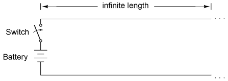
Suppose, though, that we had a set of parallel wires of infinite length, with no lamp at the end. What would happen when we close the switch? Being that there is no longer a load at the end of the wires, this circuit is open. Would there be no current at all?

  

Transmission line-Circuits and the speed of light-Part-B

Circuits and the speed of light

Suppose we had a simple one-battery, one-lamp circuit controlled by a switch. When the switch is closed, the lamp immediately lights. When the switch is opened, the lamp immediately darkens:

Transmission line- 50-Ohm Cable- Part-A

 I came across a length of coaxial cable with the label "50 ohms" printed along its outer sheath. Now, coaxial cable is a two-conductor cable made of a single conductor surrounded by a braided wire jacket, with a plastic insulating material separating the two. As such, the outer (braided) conductor completely surrounds the inner (single wire)

Effects of High VoltageTransmission Lines on Humans and Plants

Effects of High VoltageTransmission Lines 

 Introduction:

By increasing population of the world, towns are expanding, many buildings construct near high voltage overhead power transmission lines. The increase of power demand has increased the need for transmitting huge amount of power over long distances. Large transmission lines configurations with high voltage and current levels generate large values of electric and magnetic fields stresses which affect the human being and the nearby objects located at ground surfaces. This needs to be investigating the effects of electromagnetic fields near the transmission lines on human health.